Automatic Differentiation Based on Computation Graph

Automatic differentiation (AD), also called algorithmic differentiation or simply “autodiff” is one of the basic algorithms hidden behind the deep learning framework such as tensorflow, pytorch, mxnet, etc. It’s AD technique that allows us to focus on the design of the model structure without paying much attention to the gradient calculations during model training. However, this blog post will focus on the principle and implementation of AD. Finally, we will implement an AD framework based on computational graphs and use it for logistic regression. You could find all the code here.

Overview of AD

Methods for the computation of derivatives in computer programs can be classified into four categories^[2]:

1. Manually working out derivatives and coding them;
2. Numerical differentiation using finite difference approximations;
3. Symbolic differentiation using expression manipulation in computer algebra systems such as Mathematica, Maxima, and Maple;
4. Automatic differentiation, also called algorithmic differentiation.

Here, I will give a simple example to illustrate the difference between the first three methods of derivation. As for automatic differentiation, the details will be described in later sections. Suppose we need to calculate the gradient of $x=1$ for the function $ f(x)=x(1-2x)^2 $. The calculation process of different methods is as follows:

• Method 1：
  $$ f(x)=x-4x^2+4x^3 $$
  $$ f’(x)=1-8x+12x^2 $$
  $$ f’(1)=5 $$
• Method 2 ($ h $ can be any other minimum value):
  $$ f’(x) \approx \frac{f(x-h)+f(x+h)}{2h}=\frac{f(1-0.00001)+f(1+0.00001)}{2*0.00001}=5.000003999999669 $$
• Method 3:
  $$ f’(x)=(1-2x)^2 -4x(1-2x) $$
  $$ f’(1)=5 $$

From this simple example we can see the shortcomings of the first three methods. Manual differentiation is time consuming and prone to error. Numerical differentiation is simple to implement but can be highly inaccurate and calculation consuming. Symbolic differentiation addresses the weaknesses of both the manual and numerical methods, but often results in complex and cryptic expressions plagued with the problem of “expression swell”.

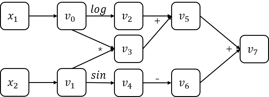
Although AD provide numerical values of derivatives and and it does so by using symbolic rules of differentiation, AD is either a type of numerical or symbolic differentiation. In order to implement the AD, we usually need to build a computation graph. Below is the computation graph of the example $ f(x_1, x_2)=log(x_1) + x_1x_2-sin(x_2) $.

Based on computation graph, there are two methods to implement AD: forward mode and reverse mode. AD in forward mode is the conceptually most simple type. For writing convenience, let $ \dot{v_i}=\frac{\partial v_i}{\partial x_1} $. So we can calculate the gradients in forward mode.

Forward Primal Trace	Forward Derivative Trace
$$ v_0=x_1=2 $$ $$ v_1=x_2=5 $$	$$ \dot{v_0}=\dot{x_1}=1 $$ $$ \dot{v_1}=\dot{x_2}=0 $$
$$ v_2=log(v_0)=log2 $$ $$ v_3=v_0v_1=10 $$ $$ v_4=sin(v1)=sin5 $$ $$ v_5=v_2+v_3=0.693+10 $$ $$ v_6=-v_4=-sin5 $$ $$ v_7=v_5+v_6=10.693+0.959 $$	$$ \dot{v_2}=\dot{v_0}/v_0=1/2 $$ $$ \dot{v_3}=\dot{v_0}v_1 + v_0\dot{v_1}=5 $$ $$ \dot{v_4}=cos(v_1)\dot{v_1}=0 $$ $$ \dot{v_5}=\dot{v_2} + \dot{v_3}=5.5 $$ $$ \dot{v_6}=-\dot{v_4}=0 $$ $$ \dot{v_7}=\dot{v_5} + \dot{v_6}=5.5 $$
$$ y=v_7=11.652 $$	$$ \dot{y}=\dot{v_7}=5.5 $$

Reverse mode is similar to forward mode, except that the gradient needs to be calculated backwards. Let $\bar{v_i}=\frac{\partial y}{\partial v_i}$. We can calculate the gradients in reverse mode.

Forward Primal Trace	Reverse Derivative Trace
$$ v_0=x_1=2 $$ $$ v_1=x_2=5 $$	$$ \bar{v_0}=\bar{v_0}^{(1)} + \bar{v_0}^{(2)}=5.5 $$ $$ \bar{v_0}^{(1)}=\bar{v_2}\frac{\partial v_2}{\partial v_0}=\frac{1}{2} $$ $$ \bar{v_0}^{(2)}=\bar{v_3}\frac{\partial v_3}{\partial v_=}=5 $$ $$ \bar{v_1}=\bar{v_4}\frac{\partial v_4}{\partial v_1}=-cos5 $$
$$ v_2=log(v_0)=log2 $$ $$ v_3=v_0v_1=10 $$ $$ v_4=sin(v1)=sin5 $$ $$ v_5=v_2+v_3=0.693+10 $$ $$ v_6=-v_4=-sin5 $$ $$ v_7=v_5+v_6=10.693+0.959 $$	$$ \bar{v_2}=\bar{v_5}\frac{\partial v_5}{\partial v_2}=1 $$ $$ \bar{v_3}=\bar{v_5}\frac{\partial v_5}{\partial v_3}=1 $$ $$ \bar{v_4}=\bar{v_6}\frac{\partial v_6}{\partial v_4}=-1 $$ $$ \bar{v_5}=\bar{v_7}\frac{\partial v_7}{\partial v_5}=1 $$ $$ \bar{v_6}=\bar{v_7}\frac{\partial v_7}{\partial v_6}=1 $$ $$ \bar{v_7}=\frac{\partial v_7}{\partial v_7}=1 $$
$$ y=v_7=11.652 $$	$$ \bar{y}=\bar{v_7}=1 $$

The above two tables demonstrate AD based on forward mode and reverse mode, respectively. Only the gradient for $ x_1 $ is calculated in the tables, and the gradient calculation for $ x_2 $ is similar, I don’t want to repeat it.

AD algorithm

The idea of the reverse mode is closer to backpropagation and is easier to program. Therefore, in practice we usually use reverse mode to implemente AD. The pseudo-code of AD based on the reverse mode is as follows:

def gradient(output_node):
    node_to_grad = {}
    node_to_grad[output_node] = 1
    # Get the reverse order topological arrangement of the nodes in computation graph
    reverse_topo_order = reversed(find_topo_sort(output_node))
    for node in reverse_topo_order:
        grad <-- sum partial adjoints from output edges of node
        # calculate the gradient of the inputs
        input_grads <-- node.op.gradient(node, grad)
        add input_grads to node_to_grad
    return node_to_grad

To better understand this algorithm, let’s look at a concrete example (You can find the implementation of this example in the test_exp function of the autodiff_test.py file).

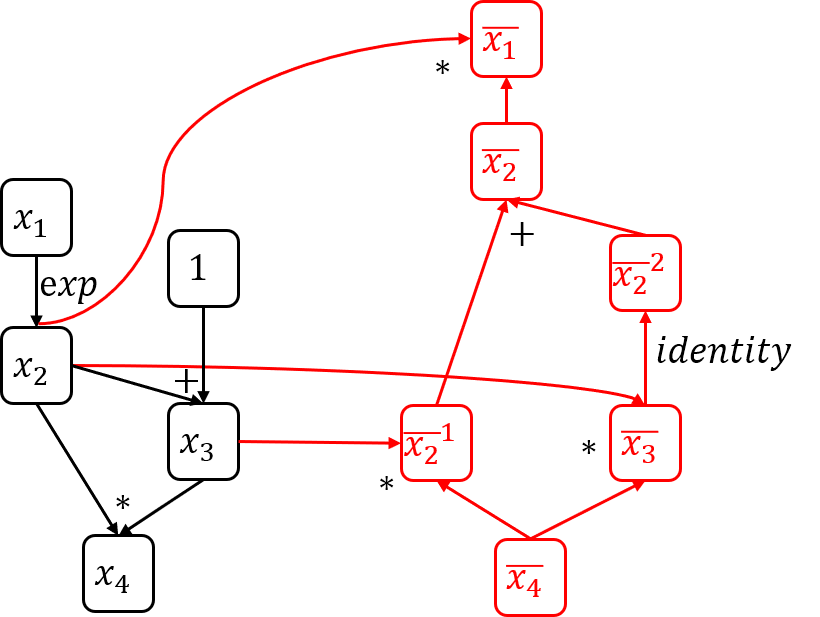
As shown in the computation graph above, the execution flow after calling function $ gradient(x_4) $ is as follows:

• Changes in node_to_grad during execution (assume $ x_1=2 $):
  1. $ x_4: \bar{x_4}=1 $;
  2. $ x_3: \bar{x_3}=\bar{x_4}x_2=e^2 $;
  3. $ x_2: \bar{x_2}^{(1)}=\bar{x_4}x_3=e^2+1 $;
  4. $ x_2: \bar{x_2}^{(2)}=\bar{x_3}=e^2 $;
  5. $ x_1: \bar{x_1}=\bar{x_2}x_2=(\bar{x_2}^{(1)} + \bar{x_2}^{(2)})x_2=e^2(2e^2+1) $.

Implementation

In order to implement AD, we first need to build a computation graph which is composed of nodes. Each node has its inputs and operation (OP). The inputs records the node or constant that entered the current node, and there may be one or more. The OP records the type of operation of the current node on the input nodes, which may be addition, subtraction, multiplication, division, or any custom mathematical operation. Below is the Python code for node.

class Node(object):
    """Node in a computation graph."""
    def __init__(self):
        """Constructor, new node is indirectly created by Op object __call__ method."""
        self.inputs = []
        self.op = None
        self.const_attr = None
        self.name = ""

    def __add__(self, other):
        """Adding two nodes return a new node."""
        if isinstance(other, Node):
            new_node = add_op(self, other)
        else:
            # Add by a constant stores the constant in the new node's const_attr field.
            # 'other' argument is a constant
            new_node = add_byconst_op(self, other)
        return new_node

    def __sub__(self, other):
        """subtracting two nodes return a new node."""
        if isinstance(other, Node):
            new_node = add_op(self, -1 * other)
        else:
            new_node = add_byconst_op(self, -1 * other)
        return new_node

    def __rsub__(self, other):
        """allow left-hand-side subtract"""
        return -1 * self.__sub__(other)

    def __mul__(self, other):
        """Multiplying to nodes return a new node."""
        if isinstance(other, Node):
            new_node = mul_op(self, other)
        else:
            new_node = mul_byconst_op(self, other)
        return new_node

    # Allow left-hand-side add and multiply.
    __radd__ = __add__
    __rmul__ = __mul__

    def __str__(self):
        """Allow print to display node name.""" 
        return self.name

    __repr__ = __str__

Each node has an OP that represents the mathematical operations that need to be performed. All OPs have a common base class. Its class definition is as follows:

class Op(object):
    """Op represents operations performed on nodes."""
    def __call__(self):
        """Create a new node and associate the op object with the node."""
        new_node = Node()
        new_node.op = self
        return new_node

    def compute(self, node, input_vals):
        """Given values of input nodes, compute the output value."""
        raise NotImplementedError

    def gradient(self, node, output_grad):
        """Given value of output gradient, compute gradient contributions to each input node."""
        raise NotImplementedError

In order to implement the corresponding mathematical operations on the node, it is only necessary to inherit the class Op and implement the function compute and gradient. In order to better explain the writing of OPs, I will write an example of the addition OP. The rest of the popular OPs will not be listed here, you can see the detailed code here. For the addition OP, there are two cases, one is to add two nodes, and the other is to add a node to a constant. Although there is only a slight difference between the two cases, we still need to treat them differently. Addition OP of two nodes is shown below:

class AddOp(Op):
    """Op to element-wise add two nodes."""
    def __call__(self, node_A, node_B, name=None):
        new_node = Op.__call__(self)
        new_node.inputs = [node_A, node_B]
        if name is not None:
            new_node.name = name
        else:
            new_node.name = "(%s+%s)" % (node_A.name, node_B.name)
        return new_node

    def compute(self, node, input_vals):
        """Given values of two input nodes, return result of element-wise addition."""
        assert len(input_vals) == 2
        return input_vals[0] + input_vals[1]

    def gradient(self, node, output_grad):
        """Given gradient of add node, return gradient contributions to each input."""
        return [output_grad, output_grad]

Addition OP of a node and a constent is shown below:

class AddByConstOp(Op):
    """Op to element-wise add a nodes by a constant."""
    def __call__(self, node_A, const_val, name=None):
        new_node = Op.__call__(self)
        new_node.const_attr = const_val
        new_node.inputs = [node_A]
        if name is not None:
            new_node.name = name
        else:
            new_node.name = "(%s+%s)" % (node_A.name, str(const_val))
        return new_node

    def compute(self, node, input_vals):
        """Given values of input node, return result of element-wise addition."""
        assert len(input_vals) == 1
        return input_vals[0] + node.const_attr

    def gradient(self, node, output_grad):
        """Given gradient of add node, return gradient contribution to input."""
        return [output_grad]

You can extend the OPs by mimicking the addition OP. In the next section, I will complete the OPs that logistic regression needs. And using the automatic differential logistic regression model for handwritten digit recognition.

After building the computation graph, we need to calculate it. The calculation of the computation graph includes the forward propagation calculation and the backward propagation (gradient) calculation. The topological ordering of the computational graph is required for any calculation. Here we use a simple post-order DFS algorithm to get the topological order.

def find_topo_sort(node_list):
    """Given a list of nodes, return a topological sort list of nodes ending in them.
    
    A simple algorithm is to do a post-order DFS traversal on the given nodes, 
    going backwards based on input edges. Since a node is added to the ordering
    after all its predecessors are traversed due to post-order DFS, we get a topological
    sort.

    """
    visited = set()
    topo_order = []
    for node in node_list:
        topo_sort_dfs(node, visited, topo_order)
    return topo_order


def topo_sort_dfs(node, visited, topo_order):
    """Post-order DFS"""
    if node in visited:
        return
    visited.add(node)
    for n in node.inputs:
        topo_sort_dfs(n, visited, topo_order)
    topo_order.append(node)

After the topological sorting of the computation graph is obtained, it can be calculated. The forward propagation calculation is wrapped in the class Executor, the code is as follows:

class Executor:
    """Executor computes values for a given subset of nodes in a computation graph.""" 
    def __init__(self, eval_node_list):
        self.eval_node_list = eval_node_list

    def run(self, feed_dict):
        """Computes values of nodes in eval_node_list given computation graph."""
        node_to_val_map = dict(feed_dict)
        # Traverse graph in topological sort order and compute values for all nodes.
        topo_order = find_topo_sort(self.eval_node_list)

        # calculated all the nodes in the computation graph.
        for node in topo_order:
            inputs = [node_to_val_map[i] for i in node.inputs]
            if inputs:
                node_to_val_map[node] = node.op.compute(node, inputs)

        # Collect node values.
        node_val_results = [node_to_val_map[node] for node in self.eval_node_list]
        return node_val_results

The specific algorithm for backpropagation has already been mentioned before. The corresponding Python code is as follows.

def gradients(output_node, node_list):
    """Take gradient of output node with respect to each node in node_list."""
    # a map from node to a list of gradient contributions from each output node
    node_to_output_grads_list = {}
    # Special note on initializing gradient of output_node as oneslike_op(output_node):
    # We are really taking a derivative of the scalar reduce_sum(output_node)
    # instead of the vector output_node. But this is the common case for loss function.
    node_to_output_grads_list[output_node] = [oneslike_op(output_node)]
    # a map from node to the gradient of that node
    node_to_output_grad = {}
    # Traverse graph in reverse topological order given the output_node that we are taking gradient wrt.
    reverse_topo_order = reversed(find_topo_sort([output_node]))

    for node in reverse_topo_order:
        output_grad = sum_node_list(node_to_output_grads_list[node])
        node_to_output_grad[node] = output_grad
        input_grads_list = node.op.gradient(node, output_grad)
        for i in range(len(node.inputs)):
            if node.inputs[i] not in node_to_output_grads_list:
                node_to_output_grads_list[node.inputs[i]] = []
            node_to_output_grads_list[node.inputs[i]].append(input_grads_list[i])

    # Collect results for gradients requested.
    grad_node_list = [node_to_output_grad[node] for node in node_list]
    return grad_node_list

If you need the full code, go here.

Logistic Regression

Based on the AD framework we have built, we only need to add some appropriate OPs to complete the LR model. If you don’t know much about the principles of LR, please refer to my blog post. This blog will not describe the details of LR. In fact, in order to implement LR, we only need to add two OPs, SigmoidOp and SigmoidCrossEntropyOp, on the existing basis.

def sigmoid_fun(x):
    return 1 / (1 + np.exp(-x))


class SigmoidOp(Op):
    def __call__(self, node_A, name=None):
        new_node = Op.__call__(self)
        new_node.inputs = [node_A]
        if name is not None:
            new_node.name = name
        else:
            new_node.name = "SigmoidOp(%s)" % node_A.name
        return new_node

    def compute(self, node, input_vals):
        assert len(input_vals) == 1
        return sigmoid_fun(input_vals[0])

    def gradient(self, node, output_grad):
        # Do not directly use SigmoidOp, use SigmoidCrossEntropyOp instead.
        raise NotImplementedError


class SigmoidCrossEntropyOp(Op):
    def __call__(self, node_A, node_B, name=None):
        new_node = Op.__call__(self)
        new_node.inputs = [node_A, node_B]
        if name is not None:
            new_node.name = name
        else:
            new_node.name = "SigmoidCrossEntropyOp(%s, %s)" % (node_A.name, node_B.name)
        return new_node

    def compute(self, node, input_vals):
        assert len(input_vals) == 2
        z = input_vals[0]
        y = input_vals[1]

        m, _ = z.shape
        loss = np.sum(y * np.log(sigmoid_fun(z)) + (1 - y) * np.log(1 - sigmoid_fun(z))) / m
        return np.array(loss)

    def gradient(self, node, output_grad):
        z = node.inputs[0]
        y = node.inputs[1]
        grad_A = (sigmoid_op(z) - y) * output_grad
        grad_B = zeroslike_op(node.inputs[1])
        return [grad_A, grad_B]

Then we can built an LR model to solve the handwritten digit recognition problem. Sine LR is an binary classification algrithm, we only select the number 0, 1 in mnist.

def mnist_lr(num_epochs=10, print_loss_val_each_epoch=False):
    print("Build logistic regression model...")

    W = ad.Variable(name="W")
    b = ad.Variable(name="b")
    X = ad.Variable(name="X")
    y = ad.Variable(name="y")

    z = ad.matmul_op(X, W) + b
    y_hat = ad.sigmoid_op(z)

    loss = ad.sigmoidcrossentropy_op(z, y)

    grad_W, grad_b = ad.gradients(loss, [W, b])
    executor = ad.Executor([loss, grad_W, grad_b, y_hat])

    # Read input data
    train_X, train_Y, test_X, test_Y = load_mnist_for_lr()
    print("train set num: %d" % train_X.shape[0])
    print("test set num: %d" % test_X.shape[0])

    # Set up minibatch
    batch_size = 1000
    n_train_batches = train_X.shape[0] // batch_size
    n_test_batches = test_X.shape[0] // batch_size

    print("Start training loop...")

    # Initialize parameters
    W_val = np.zeros((784, 10))
    b_val = np.zeros((10))
    X_val = np.empty(shape=(batch_size, 784), dtype=np.float32)
    y_val = np.empty(shape=(batch_size, 1), dtype=np.float32)
    test_X_val = np.empty(shape=(batch_size, 784), dtype=np.float32)
    test_y_val = np.empty(shape=(batch_size, 1), dtype=np.float32)

    lr = 1e-3
    for i in range(num_epochs):
        print("epoch %d" % i)
        for minibatch_index in range(n_train_batches):
            minibatch_start = minibatch_index * batch_size
            minibatch_end = (minibatch_index + 1) * batch_size
            X_val[:] = train_X[minibatch_start:minibatch_end]
            y_val[:] = train_Y[minibatch_start:minibatch_end]
            loss_val, grad_W_val, grad_b_val, _ = executor.run(
                feed_dict={X: X_val, y: y_val, W: W_val, b: b_val})
            # SGD update
            W_val = W_val - lr * grad_W_val
            b_val = b_val - lr * grad_b_val
        if print_loss_val_each_epoch:
                print(loss_val)

    correct_predictions = []
    for minibatch_index in range(n_test_batches):
        minibatch_start = minibatch_index * batch_size
        minibatch_end = (minibatch_index + 1) * batch_size
        test_X_val[:] = test_X[minibatch_start:minibatch_end]
        test_y_val[:] = test_Y[minibatch_start:minibatch_end]
        _, _, _, test_y_predicted = executor.run(
            feed_dict={
                X: test_X_val,
                y: test_y_val,
                W: W_val,
                b: b_val})
        correct_prediction = (test_y_predicted >= 0.5).astype(np.int) == test_y_val
        correct_predictions.extend(correct_prediction)
    accuracy = np.mean(correct_predictions)
    print("test set accuracy=%f" % accuracy)

After 10 epochs, we get 100% accuracy on the test set.

Conclusion

In this blog post, we detail the principles of AD and give specific derivation cases. On the basis of understanding the mathematical principles of AD, we used numpy to construct a simple calculation graph and implemented some basic OPs. Finally, we constructed the LR model on the calculation graph and used it for handwritten digit recognition.

So far, we have actually understood the basic principle behind the deep learning framework-AD based on computational graphs. However, we still have a long way to go before the real deep learning framework. Our numpy-based implementation is undoubtedly inefficient, and the real deep learning framework uses a variety of hardware acceleration.

GPU acceleration is very common in deep learning frameworks. If you want to learn about GPU-based acceleration technology, you can refer to Tinyflow.

Reference

[1] CSE 599W: System for ML
[2] Automatic Differentiation in Machine Learning: a Survey