Flink SQL源码 - Mini-Batch原理与实现

本文已收录在合集Apche Flink原理与实践中.

Mini-Batch是在进行有状态流处理时的一种重要优化手段, 通过在内存中攒批后再处理可以降低State访问次数, 从而提升吞吐量降低CPU资源使用. 目前, Flink SQL已经在多个场景中支持了Mini-Batch优化, 本文首先介绍Flink SQL的Mini-Batch实现原理, 在此基础上通过相关案例进一步介绍具体实现.

什么是Mini-Batch

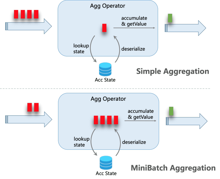
在Flink的有状态算子中, 为了保证状态的一致性, 每次操作都需要将状态保存到状态后端中, 由框架来执行Checkpoint. 然而目前RocksDB等状态的读写需要对记录进行序列化和反序列化, 甚至需要IO操作. 在这种情况下, 有状态算子很可能会成为整个作业的性能瓶颈.

为此, 对于时效性要求不是特别高, 计算状态复杂的作业可以引入Mini-Batch. 其核心思想是在内存中缓存一小批数据, 然后整批数据一起触发计算, 这样在涉及到状态访问时, 同一个Key的状态只需进行一次读写操作, 从而极大降低状态访问操作的开销, 提升作业性能. 以下是一个通过Mini-Batch进行Group Aggregate的案例(图片来自Flink文档), 通过攒批可以将4条记录的状态访问从8次减少到2次.

在Flink SQL中, 以下场景都已经支持了MiniBatch:

  • Group Aggregate
  • Top-N / Deduplicate
  • 基于Window TVF的Window Aggregate(仅有Mini-Batch实现)
  • Regular Join(在后序介绍Regular Join的文章中我们还会进一步展开)

在Flink SQL中可通过设置以下参数启用Mini-Batch.

1
2
3
4
5
6
7
8
9
// instantiate table environment
TableEnvironment tEnv = ...;

// access flink configuration
TableConfig configuration = tEnv.getConfig();
// set low-level key-value options
configuration.set("table.exec.mini-batch.enabled", "true"); // enable mini-batch optimization
configuration.set("table.exec.mini-batch.allow-latency", "5 s"); // use 5 seconds to buffer input records
configuration.set("table.exec.mini-batch.size", "5000"); // the maximum number of records can be buffered by each aggregate operator task

Mini-Batch攒批策略

Mini-Batch带来的性能提升取决于攒批的效果, 最简单的攒批方式是在需要攒批的算子上创建一个定时器, 但是这种方式对复杂的计算作业有极大限制. 举例来说, 假设用户可容忍的最大延时是10秒, 理想的攒批策略是攒10秒的数据, 然而在上述攒批方式中, 如果计算图中包含两层聚合, 那么为了保证端到端延时在10秒以内, 每层聚合最多只能攒5秒的数据, 对于聚合更多的计算图, 这种退化将更加明显.

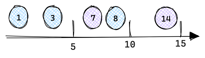
Flink在实现攒批时采用了一种更为巧妙的方法, 即使用Watermark作为批次分界. 实现上, 对于不存在Event Time的计算图, 直接在Source后添加一个MiniBatchAssigner算子, 以用户设定的延时为时间间隔下发Watermark即可; 对于存在Event Time的计算图, 为了更好的攒批, 需要将原来的Watermark按Mini-Batch时间间隔进行过滤, 仅下发能够触发每个Mini-Batch窗口的最小Watermark, 例如对于一个Watermark序列[1, 3, 7, 8, 14], 如果Mini-Batch时间间隔为5秒, 那么只需下发[7, 14]两个Watermark即可. 实现上只需在WatermarkAssigner之后新增一个MiniBatchAssigner做相应的Watermark过滤即可.

使用Watermark作为批次分界有一些明显的好处. 首先, Watermark在Flink内部已经有完善的实现机制, 通过Watermark攒批实现简单; 其次, 定时器方案会同时触发所有算子计算, 容易引起反压, 而Watermark是流动的, 攒批算子的计算是异步触发, 降低了反压风险; 最后, 使用Watermark作为批次分界还能避免数据抖动, 这种情况一般发生在两层聚合的场景下, 当内层更新时会下发-U, +U两条记录, 外层会分别处理这两条记录, 又分别下发两条-U, +U记录, 这就导致用户最终看到的结果会有一个突变的过程. 以两层聚合进行每日UV统计为例, SQL代码如下(笔者提供了可运行示例Example), 当源端收到11,2023-12-19这条记录时:

  • 内层聚合会下发-U[2023-12-19,1,1], +U[2023-12-19,1,2]两条记录;
  • 当外层聚合收到-U[2023-12-19,1,1]这条记录时会下发-U[2023-12-19,2], +U[2023-12-19,1]这两条记录, 此时2023-12-19这一天的UV值由2变为1.
  • 当外层聚合收到+U[2023-12-19,1,2]这条记录时会下发-U[2023-12-19,1], +U[2023-12-19,3]这两条记录, 此时2023-12-19这一天的UV值由1变为3.
    1
    2
    3
    4
    5
    6
    7
    8
    9
    10
    11
    12
    13
    14
    15
    16
    17
    18
    19
    20
    21
    22
    23
    24
    25
    26
    27
    28
    29
    30
    31
    32
    33
    34
    35
    36
    37
    38
    39
    /*
    输入记录
    1,2023-12-19
    2,2023-12-19
    11,2023-12-19
    */
    CREATE TABLE source (
    user_id INT,
    `day` VARCHAR
    ) WITH (...)

    /*
    关闭Mini-Batch时输出
    +----+--------------------------------+----------------------+
    | op | day | total |
    +----+--------------------------------+----------------------+
    | +I | 2023-12-19 | 1 |
    | -U | 2023-12-19 | 1 |
    | +U | 2023-12-19 | 2 |
    | -U | 2023-12-19 | 2 |
    | +U | 2023-12-19 | 1 |
    | -U | 2023-12-19 | 1 |
    | +U | 2023-12-19 | 3 |

    开启Mini-Batch时输出
    +----+--------------------------------+----------------------+
    | op | day | total |
    +----+--------------------------------+----------------------+
    | +I | 2023-12-19 | 1 |
    | -U | 2023-12-19 | 1 |
    | +U | 2023-12-19 | 2 |
    | -U | 2023-12-19 | 2 |
    | +U | 2023-12-19 | 3 |
    */
    SELECT `day`, SUM(cnt) total
    FROM (
    SELECT `day`, MOD(user_id, 10), COUNT(DISTINCT user_id) as cnt
    FROM source GROUP BY `day`, MOD(user_id, 10))
    GROUP BY `day`;

可以看到, 上述案例在统计UV值时出现了先变小后变大的过程, 尽管可以保证最终一致性, 但是下游很可能会读到一个中间值. 这一问题实际上是由前文所说的, Flink内部把UPDATE拆分为了UPDATE_BEFORE和UPDATE_AFTER两条记录所导致的. 如果用数据库中的事务来考虑, 这一拆分实际上导致了原本应该被原子执行的一个事务被分开执行了, 在ACID所定义的隔离级别中, 只能满足读未提交, 也就是说可能读到一个未提交事务的中间结果. 那为什么开启Mini-Batch之后就能避免这一问题呢? 这是由于Flink中的Watermark不会出现在UPDATE_BEFORE和UPDATE_AFTER之间, 而Watermark之间的整批数据都是一起计算的, 这样Watermark就相当于一个触发事务提交的操作, 这中间的计算对外部来说是原子的.

Table Planner处理流程

在物理关系代数(即StreamPhysicalRel)优化阶段, Table Planner会推导出当前计算图中的Mini-Batch时间间隔, 并在相应位置附上MiniBatchAssigner算子. 在Transformation图生成阶段, 会在StreamExecNode.translateToPlanInternal()中根据是否启用Mini-Batch选择对应的StreamOperator实现.

相关概念

MiniBatchInterval

MiniBatchInterval包含了Mini-Batch相关的参数, 其中interval的初始值是table.exec.mini-batch.allow-latency配置的最大容忍延时, mode表示事件时间或处理事件, 初始值是ProcTime.

1
2
3
4
5
6
7
8
9
10
11
12
public class MiniBatchInterval {
/** interval of mini-batch. */
private final long interval;
/** The type of mini-batch: rowtime/proctime. */
private final MiniBatchMode mode;
}

public enum MiniBatchMode {
ProcTime,
RowTime,
None
}

MiniBatchIntervalTrait

MiniBatchIntervalTrait是Calcite中RelTrait的一种实现, 用于标识StreamPhysicalRel节点的Mini-Batch属性. 其内部持有一个MiniBatchInterval实例, 可通过getMiniBatchInterval()方法获取.

关系代数优化阶段

在关系代数优化阶段, Mini-Batch的相关处理在physical_rewrite阶段进行. 在优化过程中:

  • 首先会通过FlinkMiniBatchIntervalTraitInitProgram为每个StreamPhysicalRel初始化MiniBatchIntervalTrait属性, 其MiniBatchInterval的初始值在StreamCommonSubGraphBasedOptimizer.doOptimize()中确定.
  • MiniBatchIntervalTrait的推导和StreamPhysicalMiniBatchAssigner节点的添加在MiniBatchIntervalInferRule中.

下面我们通过几个示例来具体介绍MiniBatchIntervalTrait的推导流程.

Processing Time Mini-Batch推导

关于Processing Time的Mini-Batch推导我们还是以文章开头的两层聚合统计每日UV为例. 它的推导流程比较简单, 经过FlinkMiniBatchIntervalTraitInitProgram初始化后, 每个StreamPhysicalRelMiniBatchIntervalTrait都是ProcTime: 5000(即Processing Time模式, 最大延时5000毫秒). MiniBatchIntervalInferRule自上而下合并各个节点的MiniBatchIntervalTrait, 直到最后一个StreamPhysicalCalc由于输入节点是StreamPhysicalTableSourceScan, 因此会插入一个StreamPhysicalMiniBatchAssigner节点. 推导前后的关系代数结构变化如下所示.

1
2
3
4
5
6
7
8
9
10
11
12
13
14
15
16
17
18
StreamPhysicalSink(table=[*anonymous_collect$1*], fields=[day, total])
StreamPhysicalGroupAggregate(groupBy=[day], select=[day, SUM_RETRACT(cnt) AS total])
StreamPhysicalExchange(distribution=[hash[day]])
StreamPhysicalCalc(select=[day, cnt])
StreamPhysicalGroupAggregate(groupBy=[day, EXPR$1], select=[day, EXPR$1, COUNT(DISTINCT user_id) AS cnt])
StreamPhysicalExchange(distribution=[hash[day, EXPR$1]])
StreamPhysicalCalc(select=[day, MOD(user_id, 10) AS EXPR$1, user_id])
StreamPhysicalTableSourceScan(table=[[default_catalog, default_database, source]], fields=[user_id, day])

StreamPhysicalSink(table=[*anonymous_collect$1*], fields=[day, total])
StreamPhysicalGroupAggregate(groupBy=[day], select=[day, SUM_RETRACT(cnt) AS total])
StreamPhysicalExchange(distribution=[hash[day]])
StreamPhysicalCalc(select=[day, cnt])
StreamPhysicalGroupAggregate(groupBy=[day, EXPR$1], select=[day, EXPR$1, COUNT(DISTINCT user_id) AS cnt])
StreamPhysicalExchange(distribution=[hash[day, EXPR$1]])
StreamPhysicalCalc(select=[day, MOD(user_id, 10) AS EXPR$1, user_id])
StreamPhysicalMiniBatchAssigner(interval=[5000ms], mode=[ProcTime])
StreamPhysicalTableSourceScan(table=[[default_catalog, default_database, source]], fields=[user_id, day])

Event Time Mini-Batch推导

在Event Time场景中, 我们来看一个更加复杂的例子, 其计算图结构如下所示, 在Deduplicate之后存在两个Tumbling窗口聚合操作, 其中一个窗口大小为5s, 另一个为10s. 此时, 若table.exec.mini-batch.allow-latency所设延时为15s, 那么最终MiniBatchAssigner的延迟应该为多少呢?

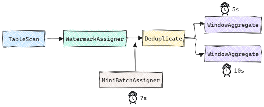
目前Flink Table Planner的实现中, 并没有考虑窗口大小对Mini-Batch的影响, 也就是说上述案例的MiniBatchAssigner延迟为15s(读者可运行MiniBatchEventTimeExample获得更直观的感受). 从语义上来说并没有问题, 因为用户所能容忍的最大延时是15s. 但是, 如果MiniBatchAssigner的延时远大于窗口大小, 那么会导致在某一时刻触发大量窗口计算. 在这种情况下, 更合理的方案应该是以窗口大小的最大公约数为MiniBatchAssigner延迟(上述案例中即为5s).

Transformation图生成阶段

在Transformation图生成阶段与Mini-Batch相关的有两个方面:

  • 一是需要将StreamPhysicalMiniBatchAssigner转换为对应的StreamOperator实现, 这一步在StreamExecMiniBatchAssigner中实现.
  • 二是需要将对应支持Mini-Batch的算子转换Mini-Batch实现, 这一步在算子的StreamExecNode.translateToPlanInternal()中实现. 下文中我们以Group Aggregate为例, 具体介绍攒批算子的实现.

MiniBatchAssginerOperator实现

MiniBatchAssginerOperator在Event Time和Processing Time场景下有不同的实现.

Event Time场景下的实现在RowTimeMiniBatchAssginerOperator中, 主要代码如下, 核心逻辑就是在processWatermark()中拦截上游产生的Watermark, 对其进行过滤, 最终仅下发能否出发Mini-Batch批次的最小Watermark.

1
2
3
4
5
6
7
8
9
10
11
12
13
14
15
16
17
18
19
20
21
22
23
24
25
26
27
28
29
30
31
32
public class RowTimeMiniBatchAssginerOperator extends AbstractStreamOperator<RowData>
implements OneInputStreamOperator<RowData, RowData> {

@Override
public void processWatermark(Watermark mark) throws Exception {
// if we receive a Long.MAX_VALUE watermark we forward it since it is used
// to signal the end of input and to not block watermark progress downstream
if (mark.getTimestamp() == Long.MAX_VALUE && currentWatermark != Long.MAX_VALUE) {
currentWatermark = Long.MAX_VALUE;
output.emitWatermark(mark);
return;
}

currentWatermark = Math.max(currentWatermark, mark.getTimestamp());
// 仅当当前Watermark大于下一个批次窗口触发时间时推进
if (currentWatermark >= nextWatermark) {
advanceWatermark();
}
}

private void advanceWatermark() {
output.emitWatermark(new Watermark(currentWatermark));
// 计算Mini-Batch批次的开始和结束时间
long start = getMiniBatchStart(currentWatermark, minibatchInterval);
long end = start + minibatchInterval - 1;
nextWatermark = end > currentWatermark ? end : end + minibatchInterval;
}

private static long getMiniBatchStart(long watermark, long interval) {
return watermark - (watermark + interval) % interval;
}
}

Processing Time场景下的实现在ProcTimeMiniBatchAssignerOperator中, 主要代码如下. 在processElement()会判断当前时间是否可以出发一个Batch, 如果可以则会下发一个Watermark. 如果没有持续的数据输入, onProcessingTime()会保证每隔一个Mini-Batch窗口下发一个Watermark.

1
2
3
4
5
6
7
8
9
10
11
12
13
14
15
16
17
18
19
20
21
22
23
24
25
26
27
28
public class ProcTimeMiniBatchAssignerOperator extends AbstractStreamOperator<RowData>
implements OneInputStreamOperator<RowData, RowData>,
ProcessingTimeService.ProcessingTimeCallback {

@Override
public void processElement(StreamRecord<RowData> element) throws Exception {
long now = getProcessingTimeService().getCurrentProcessingTime();
long currentBatch = now - now % intervalMs;
if (currentBatch > currentWatermark) {
currentWatermark = currentBatch;
// emit
output.emitWatermark(new Watermark(currentBatch));
}
output.collect(element);
}

@Override
public void onProcessingTime(long timestamp) throws Exception {
long now = getProcessingTimeService().getCurrentProcessingTime();
long currentBatch = now - now % intervalMs;
if (currentBatch > currentWatermark) {
currentWatermark = currentBatch;
// emit
output.emitWatermark(new Watermark(currentBatch));
}
getProcessingTimeService().registerTimer(currentBatch + intervalMs, this);
}
}

攒批计算

Group Aggregate的攒批计算是由AbstractMapBundleOperatorMapBundleFunction配合完成的, Top-N和Deduplicate的实现也类似, 只不过有各自具体的实现. 不过基于Window TVF实现的Window Aggregate有一套独立的攒批逻辑, 具体在后续文章中进一步介绍.

AbstractMapBundleOperator继承自StreamOperator, 它有两个实现类, 分别用于keyed-stream和non-keyed-stream. 实际上核心的处理逻辑都实现在AbstractMapBundleOperator中.

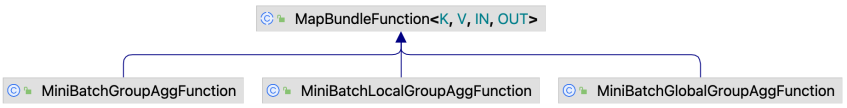
MapBundleFunction有三个实现类与Group Aggregate相关, 其中MiniBatchGroupAggFunction用在未开启Local-Global Aggregation的场景; MiniBatchLocalGroupAggFunction用在Local聚合阶段; MiniBatchGlobalGroupAggFunction用在Global聚合阶段.

下面我们介绍在不开启Local-Global优化时的实现, 其核心代码如下.

1
2
3
4
5
6
7
8
9
10
11
12
13
14
15
16
17
18
19
20
21
22
23
24
25
26
27
28
29
30
31
32
33
34
35
36
37
38
39
40
41
42
43
44
45
46
47
48
49
50
51
52
53
54
55
56
57
58
59
60
61
62
63
64
public abstract class AbstractMapBundleOperator<K, V, IN, OUT> extends AbstractStreamOperator<OUT>
implements OneInputStreamOperator<IN, OUT>, BundleTriggerCallback {

@Override
public void processElement(StreamRecord<IN> element) throws Exception {
// get the key and value for the map bundle
final IN input = element.getValue();
final K bundleKey = getKey(input);
final V bundleValue = bundle.get(bundleKey);

// get a new value after adding this element to bundle
// function是MiniBatchGroupAggFunction实例
final V newBundleValue = function.addInput(bundleValue, input);

// update to map bundle
// bundle是一个内存Map, 用于在内存中保存整批数据
bundle.put(bundleKey, newBundleValue);

numOfElements++;
// bundleTrigger是一个CountBundleTrigger实例,
// 当批次数据条数达到table.exec.mini-batch.size所设值时便会触发finishBundle()计算
bundleTrigger.onElement(input);
}

@Override
public void finishBundle() throws Exception {
if (bundle != null && !bundle.isEmpty()) {
numOfElements = 0;
function.finishBundle(bundle, collector);
bundle.clear();
}
bundleTrigger.reset();
}

@Override
public void processWatermark(Watermark mark) throws Exception {
// 在处理Watermark时也触发计算, 因为Watermark是批次分界
finishBundle();
super.processWatermark(mark);
}
}

public class MiniBatchGroupAggFunction
extends MapBundleFunction<RowData, List<RowData>, RowData, RowData> {

@Override
public List<RowData> addInput(@Nullable List<RowData> value, RowData input) throws Exception {
List<RowData> bufferedRows = value;
if (value == null) {
bufferedRows = new ArrayList<>();
}
// input row maybe reused, we need deep copy here
bufferedRows.add(inputRowSerializer.copy(input));
return bufferedRows;
}

@Override
public void finishBundle(Map<RowData, List<RowData>> buffer, Collector<RowData> out)
throws Exception {
// 这里的实现逻辑与GroupAggFunction.processElement()逻辑类似
// 在之前的博文中已经介绍过(https://liebing.org.cn/flink-sql-changelog.html#Transform%E5%9B%BE%E7%94%9F%E6%88%90%E9%98%B6%E6%AE%B5)
...
}
}

总结

目前Flink SQL已经在多个有状态计算场景中引入了Mini-Batch来减少计算过程中对状态的访问次数, 实际上Mini-Batch在无状态计算中也能发挥作用, 对于无状态算子, 可以通过Mini-Batch攒批后使用数据库中常用的向量化计算技术进行计算, 从而减少作业所需的CPU资源.

总结来说, Mini-Batch除了会增加一定的延时, 存在诸多的好处:

  • 对于有状态算子可以减少状态访问, 从而极大提升作业吞吐量;
  • 防止数据抖动, 同时减少下游存储写入压力;
  • 在Regular Join中可减少回撤, 从而提升双流及多流Join的性能.

参考

[1] Flink Documentation - Table API & SQL - Performance Tuning

Flink源码 - RPC原理与实现 Flink SQL源码 - Changelog原理与实现

本博客所有文章除特别声明外, 均采用CC BY-NC-SA 3.0 CN许可协议. 转载请注明出处!


关注笔者微信公众号获得最新文章推送

Comments

Your browser is out-of-date!

Update your browser to view this website correctly. Update my browser now

×